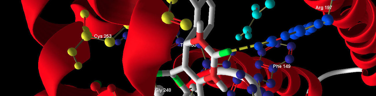
Feature Importance for Drug Discovery

In silico interpretation of compound selection using permuted feature importance of neural networks to rank High-Throughput Screening (HTS) criteria, and identify 2 compounds (out of 57,546) with 95% confidence of target activation.

💾 Data

Reference Example Datasets for more information.

This dataset is comprised of:

• Features - 155 structural screening criteria for each compound.

• Labels - whether or not the MAPK target is activated or inactivated by the compound.

  Source: PubChem Bioassay from Scripps Research Institute Molecular Screening Center. https://archive.ics.uci.edu/ml/datasets/PubChem+Bioassay+Data

The purpose of this analysis is to use permuted feature importance to understand which chemical structures are driving the activation of the target.

import pandas as pd
df = pd.read_parquet("MAPK_bioassay.parquet")

from aiqc.orm import Dataset
shared_dataset = Dataset.Tabular.from_df(df)

---

---

🚰 Pipeline

Since we have so many columns, we will examine their variation en masse in order to determine how we want to encode them.

features = df.columns.tolist()
features.remove('Outcome')

features_binary = []
features_nonbinary = []

for col in features:
    values = len(df[col].value_counts().tolist())
    if (values == 1):
        pass #no variation
    elif (values == 2):
        features_binary.append(col)
    else:
        # None appeared ordinal.
        features_nonbinary.append(col)

print(f"Binary Features = {len(features_binary)} ")
print(f"Non-binary Features = {len(features_nonbinary)} ")

Binary Features = 123
Non-binary Features = 31

Reference High-Level API Docs for more information.

from aiqc.mlops import Pipeline, Input, Target, Stratifier
from sklearn.preprocessing import LabelBinarizer, OrdinalEncoder, StandardScaler

pipeline = Pipeline(
    Input(
        dataset = shared_dataset,
        encoders = [
            Input.Encoder(OrdinalEncoder(), columns=features_binary),
            Input.Encoder(StandardScaler(), columns=features_nonbinary)
        ]
    ),

    Target(
        dataset   = shared_dataset
        , column  = 'Outcome'
        , encoder = Target.Encoder(LabelBinarizer())
    ),

    Stratifier(size_test=0.26)
)

---

🧪 Experiment

Reference High-Level API Docs for more information.

from aiqc.mlops import Experiment, Architecture, Trainer
from aiqc.utils.tensorflow import TrainingCallback
import tensorflow as tf
from tensorflow.keras import layers as l

def fn_build(features_shape, label_shape, **hp):
    m = tf.keras.models.Sequential()
    m.add(l.Input(shape=features_shape))

    # First hidden layer.
    m.add(l.Dense(
        hp['first_neurons'],
        kernel_initializer=hp['init']
    ))
    m.add(l.BatchNormalization())
    m.add(l.Activation(hp['activation']))
    m.add(l.Dropout(hp['drop_rate']))

    # Second hidden layer.
    if (hp['second_layer']==True):
        m.add(l.Dense(
            hp['after_neurons'],
            kernel_initializer=hp['init']
        ))
        m.add(l.BatchNormalization())
        m.add(l.Activation(hp['activation']))
        m.add(l.Dropout(hp['drop_rate']))

    # Output layer
    m.add(l.Dense(
        units=label_shape[0],
        activation='sigmoid',
        kernel_initializer='glorot_uniform'
    ))
    return m

def fn_train(
    model, loser, optimizer,
    train_features, train_label,
    eval_features, eval_label,
    **hp
):
    model.compile(
        loss        = loser
        , optimizer = optimizer
        , metrics   = ['accuracy', tf.keras.metrics.Precision()]
    )

    # Early stopping.
    metric_cuttoffs = [
        {"metric":"val_precision", "cutoff":0.75, "above_or_below":"above"},
    ]
    cutoffs = TrainingCallback.MetricCutoff(metric_cuttoffs)

    model.fit(
        train_features, train_label
        , validation_data = (eval_features, eval_label)
        , verbose         = 0
        , batch_size      = hp['batch_size']
        , epochs          = hp['epochs']
        , callbacks       = [tf.keras.callbacks.History()]
    )
    return model

def fn_lose(**hp):
    if (hp['loss_imbalanced']==True):
        loser = tf.keras.losses.BinaryFocalCrossentropy(gamma=hp['gamma'], from_logits=False)
    else:
        loser = tf.keras.losses.BinaryCrossentropy()
    return loser

def fn_optimize(**hp):
    optimizer = tf.keras.optimizers.Adamax(hp['learning_rate'])
    return optimizer

hyperparameters = dict(
    first_neurons     = [120]
    , after_neurons   = [12]
    , second_layer    = [True, False]
    , activation      = ['relu']
    , init            = ['he_uniform']
    , epochs          = [20]
    , batch_size      = [5]
    , drop_rate       = [0.4]
    , gamma           = [1.0]
    , loss_imbalanced = [True, False]
    , learning_rate   = [0.01]
)

queue = Experiment(
    Architecture(
        library           = "keras"
        , analysis_type   = "classification_binary"
        , fn_build        = fn_build
        , fn_train        = fn_train
        , fn_optimize     = fn_optimize
        , hyperparameters = hyperparameters
    ),

    Trainer(
        pipeline        = pipeline
        , repeat_count  = 2
        , repeat_count  = 3
        , permute_count = 7
    )
)

queue.run_jobs()

🔮 Training Models 🔮: 100%|████████████████████████████████████████| 12/12 [07:44<00:00, 38.74s/it]

---

Interpretation

id = 666
predictor = aiqc.Predictor.get_by_id(id)
prediction = predictor.predictions[0]

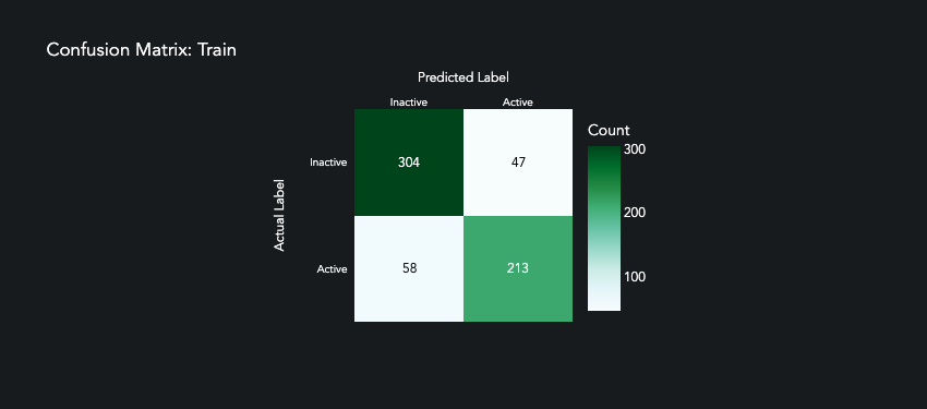
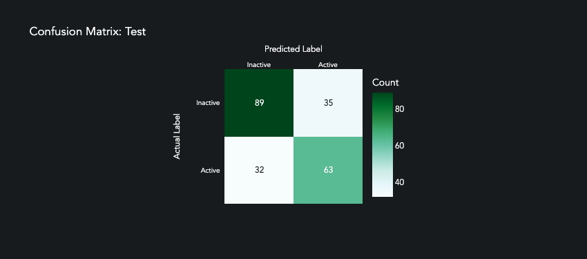
It’s not perfect, but the model has learned some of predictive patterns within the data.

prediction.plot_confusion_matrix()

The Experiment.permute_count parameter determines how many times each feature is permuted and run back through the model. The median difference in loss is then compared to the baseline loss of the model.

prediction.plot_feature_importance(height=1000)

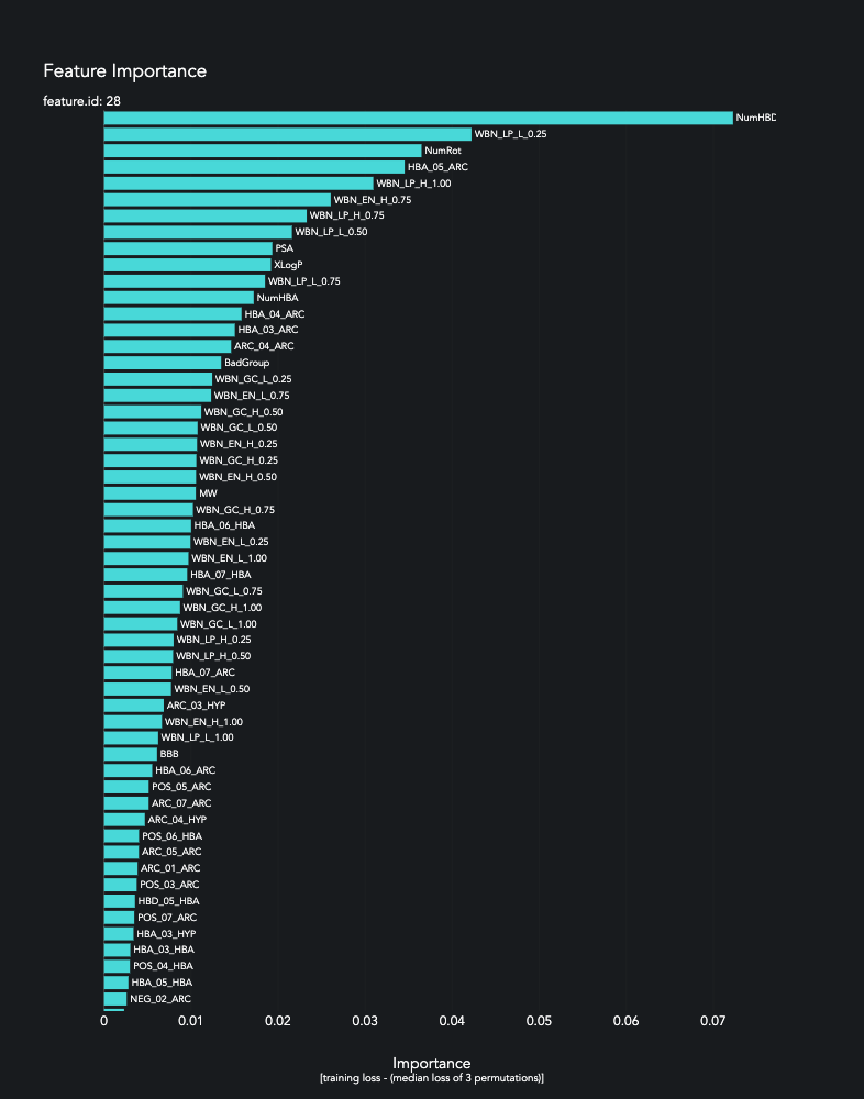
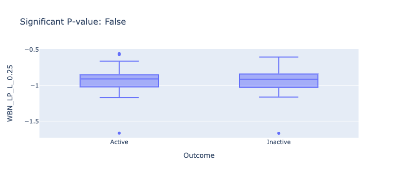
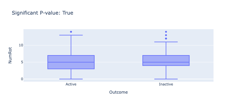
In comparison to traditional statistics, the heuristics of deep learning help us quantify the impact of subtle variation within the dataset.

• Box plots appeared nearly identical.

• T-tests did not rule all of these features to be significant.

Despite this, our model is able to achieve f1=0.726 and precision=0.735, which can help us rule out/in tens of thousands of future compounds. This suggests that the model is able to detect not only variation within a feature, but also interaction between features.

from scipy.stats import ttest_ind

active = df[df['Outcome']=='Active']
inactive = df[df['Outcome']=='Inactive']
top_6 = ['NumHBD','NumRot','WBN_LP_L_0.25','HBA_05_ARC','WBN_LP_H_1.00','WBN_EN_H_1.00']

for col in top_6:
    ttest_sig = ttest_ind(active[col], inactive[col])[1]<0.05
    px.box(df, x="Outcome", y=col, title=f"Significant P-value: {ttest_sig}", height=50).show()

Finally, our model enables us to determine which compounds most strongly fit these patterns based on the probability of their prediction.

dfs = []
for split in ['train','test']:
    sample_ids = splitset.samples[split]
    sample_probabilities = prediction.probabilities[split]

    samples = splitset.label.to_df(samples=sample_ids)
    samples['Probability'] = sample_probabilities
    samples['Compound_ID'] = sample_ids

    samples = samples[samples['Probability'] >= 0.95]
    samples = samples[samples['Outcome'] == 'Active']
    dfs.append(samples)
pd.concat(dfs)

	Outcome	Probability	Compound_ID
113	Active	0.977319	113
174	Active	0.964854	174

Across our entire dataset of 57,546 compounds, only 2 compounds exhibit over 95% probability of being active. If we trust the scientific relevance of these features, then these compounds are great candidates for the next phase.

---

Visualization & Interpretation

For more information on visualization of performance metrics, reference the Dashboard documentation.