Deep Learning 101

Boiling down a neural network to its fundamental concepts.

🔍 Types of Analysis

If you are generally familiar with spreadsheets then you are already half way to understanding AI. For the purpose of this discussion, let's assume that each row in a spreadsheet represents a record, and each column provides information about that record. Bearing this in mind, there are two major types of AI:

Generative	Given what we know about rows 1:1000 → generate row 1001.
Discriminative	Given what we know about columns A:F → determine column G’s values.

🔬 Subtypes of Analysis

In this tutorial, we will focus on discriminative analysis as it is highly practical and easier to understand. Discrimination helps us answer two important kinds of questions:

Categorize	What is it?	aka classify	e.g. benign vs malignant? which species?
Quantify	How much?	aka regress	e.g. price? distance? age? radioactivity?

Digging one level deeper, there are two types of categorization:

Binary	Checking for the presence of a single condition	e.g. tumor
Multi-Label	When there are many possible outcomes	e.g. species

🌡️ Variables

As an example, let's pretend we work at a zoo where we have a spreadsheet that contains information about the traits of different animals. We want to use discriminative learning in order to categorize the species of a given animal.

Features	Indepent Variable (X)	Informative columns like num_legs, has_wings, has_shell.
Label	Dependent Variable (y)	The species column that we want to predict.

We learn about the features in order to predict the label.

🍱 Stratification

Our predictive algorithm will need samples to learn from as well as samples for evaluating its performance.

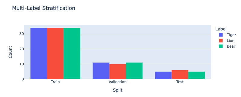
So we split our dataset into subsets for these purposes. It's important that the distribution of each subset is representatitive of the broader population because we want our algorithm to be able to generalize.

Train	67%	What the algorithm is trained on/ learns from.
Validation	21%	What the model is evaluated against during training.
Test	12%	Blind holdout for evaluating the model at the end of training.

📞 Encoding & Decoding

Data needs the be numerically encoded before it can be fed into a neural network.

Binarize	Categorical	1 means presence, 0 means absence.
OneHotEncode(OHE)	Categorical	Expand 1 multi-category col into many binary cols.
Ordinal	Categorical	[Bad form] Each category assigned an integer [0,1,2].
Scale	Continuous	Shrink the range of values between -1:1 or 0:1.

This normalization also helps features start on equal footing and prevent gradient explosion.

After the algorithm makes its prediction, that information needs to be decoded back into its orginal format so that it can be understood by practitioners.

⚖️ Algorithm

Now we need an equation (aka algorithm or model) that predicts our label when we show it a set of features. Here is our simplified example:

species = (num_legs * x) + (has_wings * y) + (has_shell * z)

This mock equation is actually identical to a neural network with neither hidden layers nor bias neurons.

The challenging part is that we need to figure out the right values (aka weights) for the parameters (x, y, z) so that our algorithm makes accurate predictions ⚖️ To do this by hand, we would simply use trial-and-error; change the value of x, and then see if that change either improved the model or made it worse.

🎢 Gradient Descent

Fortunately, computers can rapidly perform these repetetitive calculations on our behalf. This is where the magic of AI comes into play. It simply automates that trial-and-error.

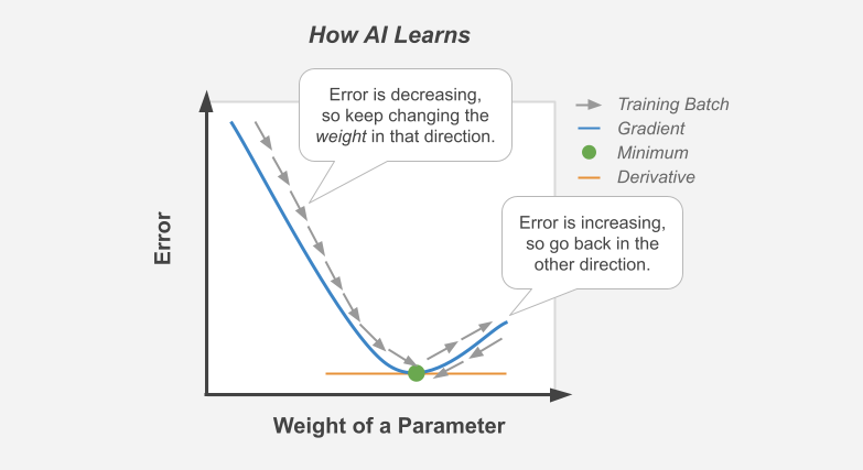
The figure above demonstrates what happens during a training batch: (1) the algorithm looks at a few rows, (2) makes predictions about those rows using its existing weights, (3) checks how accurate those predictions are, (4) adjusts its weights in an attempt to minimize future errors. It's like finding the bottom of a valley by rolling a ball down it.

With repetition, the model molds to the features like a memory foam mattress.

🏛️ Architectures

There are different types of algorithms (aka neural network architectures)
for working with different types of data:

Linear	🧮 Tabular	e.g. spreadsheets & tables.
Convolutional	📸 Positional	e.g. images, videos, & networks.
Recurrent	⏱️ Ordered	e.g. time, text, & DNA.

They can be mixed and matched to handle almost any real-life scenario.

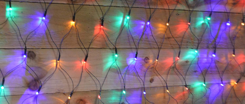
🕸️ Networks

Graph theory is a mathematical discipline that represents connected objects as networks comprised of:

Nodes	neurons	participants in the network	💡 e.g. lightbulbs
Edges	weights	connect (aka link) the nodes together	🔌 e.g. wires

🗺️ Topology

The structure of the neural network is referred to as the topology. The diagram below shows the topology of a linear architecture. Although it may seem overwhelming at first, the mechanisms of the individual components are actually quite simple. We'll start with the big picture and then deconstruct it to understand what each piece does.

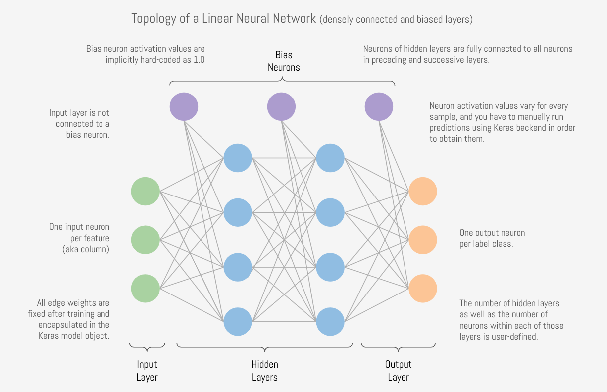
Running with our network analogy - as data passes through each wire, it is multiplied by that wire's adjustable weight that we mentioned previously. In this way, the weights act like amplifiers that adjust the voltage passing through the network. Meanwhile, the neurons are like lightbulbs with degrees of brilliance based on the strength of the voltage they receive from all of their incoming wires. The bias neurons don't actually touch the data. They act like a y-intercept (think b in y = mx + b).

If things still aren't making sense, try thinking of a neural network as a galtonboard (aka "bean machine"). The goal is to shape the topology of the network so that it can successfully tease apart the patterns in the data to make the right predictions.

🧅 Layers

Within a neural network, there are different types of layers:

Input	Receives the data. Mirrors the shape of incoming features.
Hidden	Learns from patterns in the features. The number of layers & neurons based on feature complexity.
Output	Compares predictions to the real label. Mirrors shape of labels (# of categories).
Regulatory	[Not pictured here] Dropout, BatchNorm, MaxPool keep the network balanced and help prevent overfitting.

Coming back to our zoo example, the number of input neurons in our input layer would be equal to the number of features, and the number of output neurons in our output layer would be equal to the number of possible species.

The number of hidden layers and the amount of hidden neurons in those layers will vary based on the complexity of the problem we are trying to solve 🦏 Classifying rhinos vs mosquitoes based on their weight is such a simple task that it would not require any hidden layers at all 🐆 However, delineating the subtle differences between types of big cats (lynx, ocelot, tiger, cougar, panther) may require several layers in order to tease apart their differences. For example, the first hidden layer might check for spotted vs striped fur, while the second hidden layer determines the color of that marking.

🧠 Biological Neurons

How does a neuron in the brain process information?

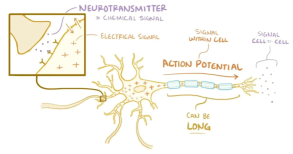
In the brain, networks of neurons work together to respond to an incoming stimulus. They repeatedly pass information to downstream neurons in the form of neurotransmitters.

However, neurons only forward information if certain conditions are met. As the neuron receives incoming signals, it builds up an electrically charged chemical concentration (aka action potential) inside its cell membrane. When this concentration exceeds a certain threshold, it fires a spike.

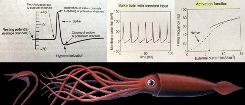
The Hodgkin-Huxley duo discovered these phenomena by observing the rate at which neurons in giant squids fired spikes based on variations in current 🦑 Trappenburg, Fundamentals of Computational Neuroscience. 2nd edition, 2010

⚡ Artificial Neurons

How does an artificial neuron process information?

Similar to how a biological neuron aggregates an action potential based on input from preceding neurons - an artificial neuron aggregates a weighted sum by adding up all of the values of its incoming weights.

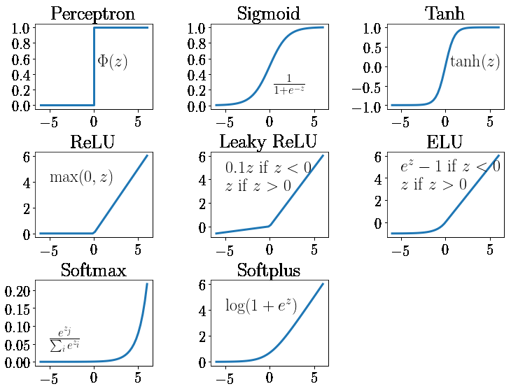
How then is the spiking threshold for artificial neurons determined? Any way we program it! The weighted sum can be ran through any activation function of our choosing.

Different layers make use of different activation functions:

Input	In a linear network, the receiving layer does not have an activation function.
Hidden	The de facto activation function is ReLU. Rarely, Tanh.
Output	Sigmoid for binary classify. Softmax for multi-label classify. None for regression.

📈 Performance Metrics

How does the algorithm know if its predictions are accurate? As mentioned in the sections above, it calculates the difference between its predicted label and the actual label. There are different strategies for calculating this loss:

BinaryCrossentropy	Binary classification.
CategoricalCrossentropy	Multi-label classification.
MeanSquaredError or MeanAbsoluteError.	Used for regression.

Although neural networks are great at minimizing loss, this metric is hard for humans to understand. The following two metrics are easy to understand because they both max out at 1.0 aka 100%:

Accuracy	Classification.
R²	Regression.

A learning curve keeps track of these metrics over the course of model training:

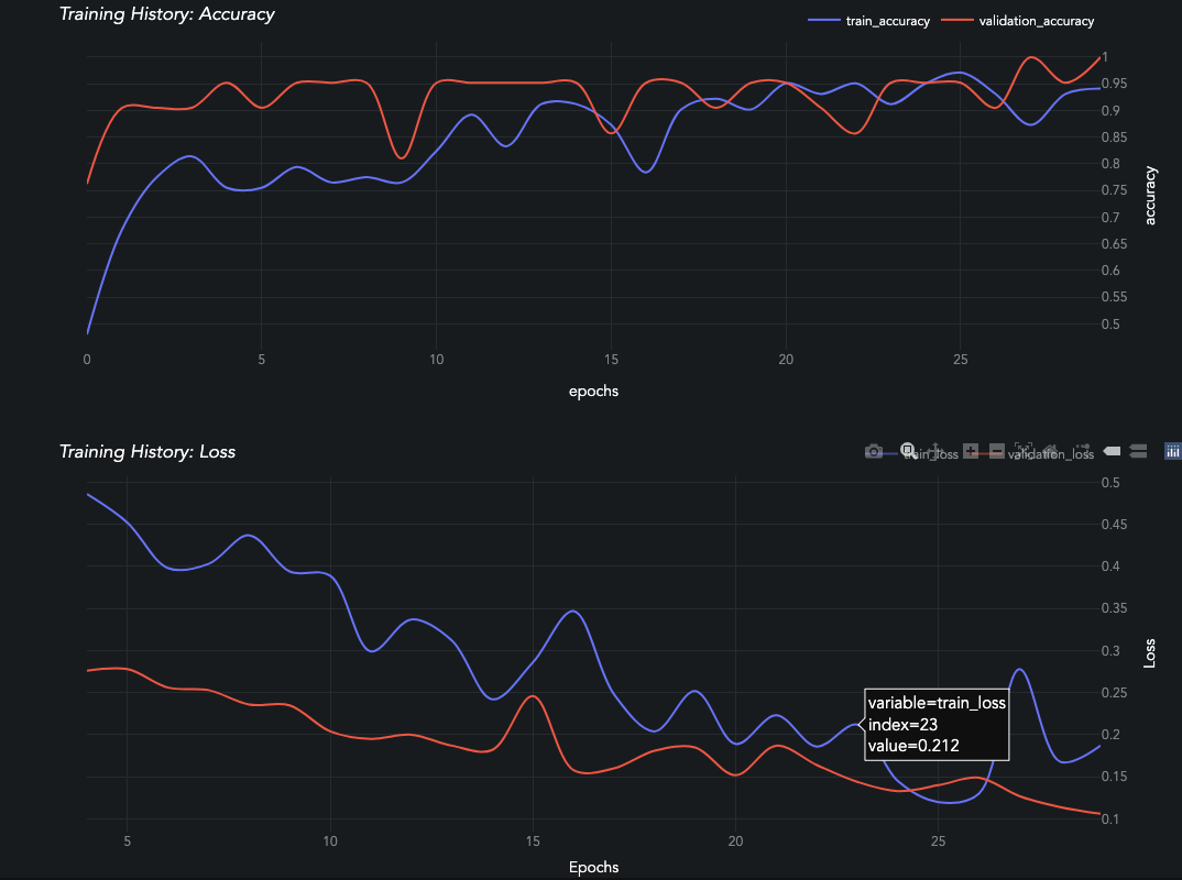
Have a look at the other visualizations & metrics provided by AIQC.

🎛️ Tuning

A data scientist oversees the training of an neural network much like a chef prepares a meal. The heat is what actually cooks the food, but there are still a few things that the chef controls:

Duration	Food isn’t fully cooked? Train for more epochs or decrease the size of each batch.
Parameters	Burning? Turn down learning rate. Tastes bad? Try initialization/ activation spices.
Topology	If the food doesn’t fit in the pan, switch to a larger pan with deeper/ taller layers.
Regulation	Overfitting on the same old recipes? Add more Dropout to mix things up.

At first, the number of tuning options seems overwhelming, but you quickly realize that you only need to learn a handful of common dinner recipes in order to get by.

🚀 Let's Get Started

Now you're ready to start your own experiments with the help of the tutorials. The rest is just figuring out how to feed your data into and out of the algorithms, which is where the AIQC framework comes into play.

The classic xkcd comic.

→ Use Cases & Tutorials